We are currently working on a project for a UK water company which involves building DMA models to conduct network analysis. As part of this process, we have found that concepts from graph theory can be applied both to facilitate data cleansing activities and provide insight into the nature and expected behaviour of a water network.
This blog post aims to introduce some of these concepts and demonstrate how they can be applied, with examples using the Python package Networkx.
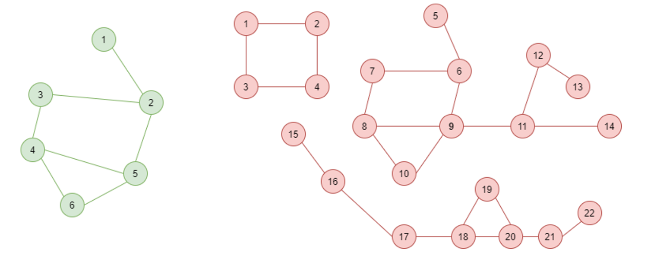
Graph theory is an area of mathematics concerned with ‘graphs’. Graphs can be defined as mathematical structures used to model pairwise relations between objects, made up of vertices (also called nodes or points) which are connected by edges (also called links or lines). Two simple example graphs are shown in Figure 1.
Figure 1a: A simple, connected graph Figure 1b: A graph with three components
Graph theory is widely utilised in satellite navigation software for route planning by representing the road network as a graph, where the junctions are represented by nodes and the roads are represented by links between them. But how can it be applied to a water network? If the reader is familiar with hydraulic network modelling, the use of the words ‘links’ and ‘nodes’ above might highlight some parallels between the two fields.
There are several data structures which can be used to represent a graph. Networkx conveniently allows graphs to be built from an edge-list (a list of node pairs which denotes that each pair is connected). In our case, this makes it possible to graph a DMA by running an SQL query which returns an edge-list where each ‘edge’ (or link) represents a pipe. Having used this to write a standard graph_dma(dma) function, we explored what functionality in Networkx might provide us with some insight by analysing the DMA graphs.
Network connectivity
A basic concept in graph theory is ‘connectedness’, or whether or not every node in the graph is connected by some route to every other node. For example, figure 1 shows two simple graphs where figure 1a is connected, but figure 1b is not. The graph in figure 1b contains three separate ‘components’ (distinct sub-graphs which are themselves connected but which are not inter-connected). Based on these concepts, Networkx provides useful functions which can be used to help assess connectivity issues within model data. The function is_connected(G) is a simple Boolean check of whether a DMA has any connectivity issues. This is useful as a data health check, but how do we deal with those areas where issues have been identified?
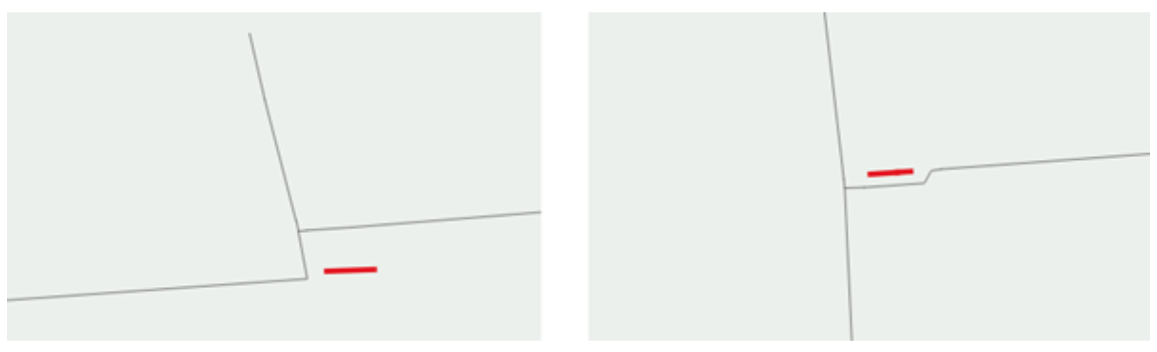
By using the function connected_components(G) we can count how many distinct sub-graphs there are within a DMA and sum the mains length within each as a measure of the extent of the network data issues. By combining this with a query counting the number of properties fed from pipes in each component, we have been able to implement an automated data cleansing procedure to detect small disconnected portions of network which do not feed any properties (see Figures 2a & 2b) and automatically delete them. This is invaluable to remove stray or incorrectly drawn pipes imported from the client GIS data which could otherwise prevent a model from solving successfully.
Figures 2a & 2b: Two separate examples of pipes (shown in red) deleted by automated routine
Floating assets
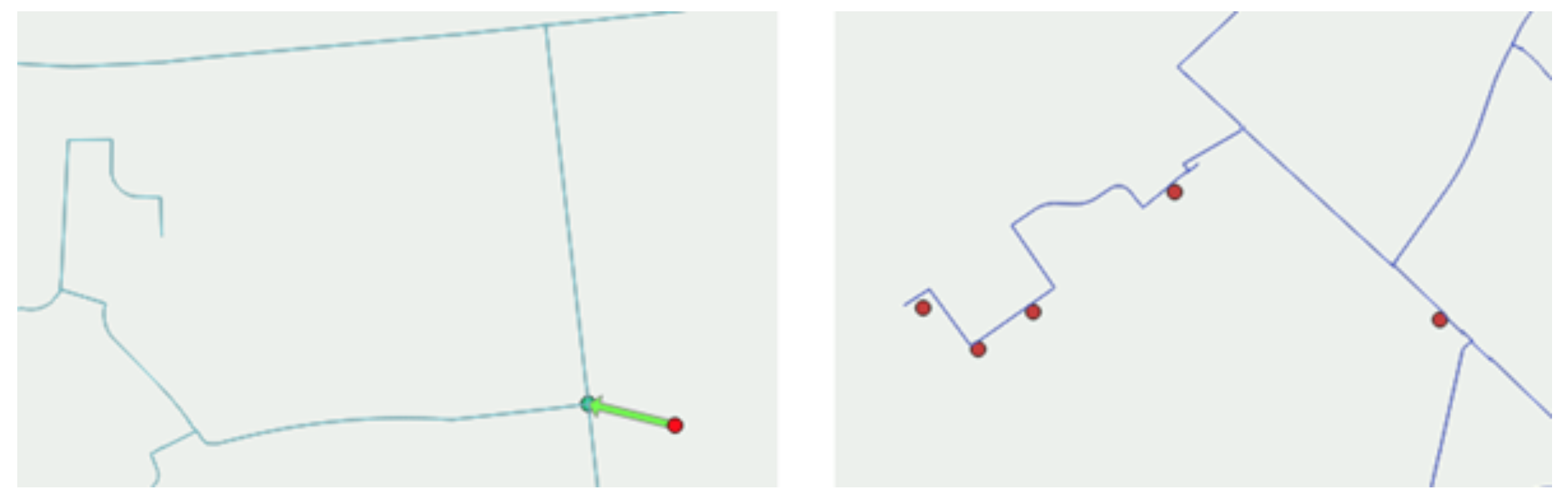
Another common GIS data issue is that some assets (e.g. valves, hydrants and meters) are ‘floating’ over or near to the pipes, rather than connected into the network. In graph theory, a node is termed an ‘isolate’ if it is not connected by an edge to any other node in the graph. By using the function isolates(G) we can identify the assets which are not properly connected into the network and that would prevent a model from running, and deal with them automatically based on their type.
Figure 3 shows some example results from this clean up. The hydrant in Figure 3a is pressure monitored as part of our project fieldwork and therefore required to be in the model, so it has been attached to the nearest suitable location. The open valves in Figure 3b (shown in red) are extraneous to the function of the model as they are associated with minor customer connections rather than network isolation and have therefore been automatically deleted.
Branched networks
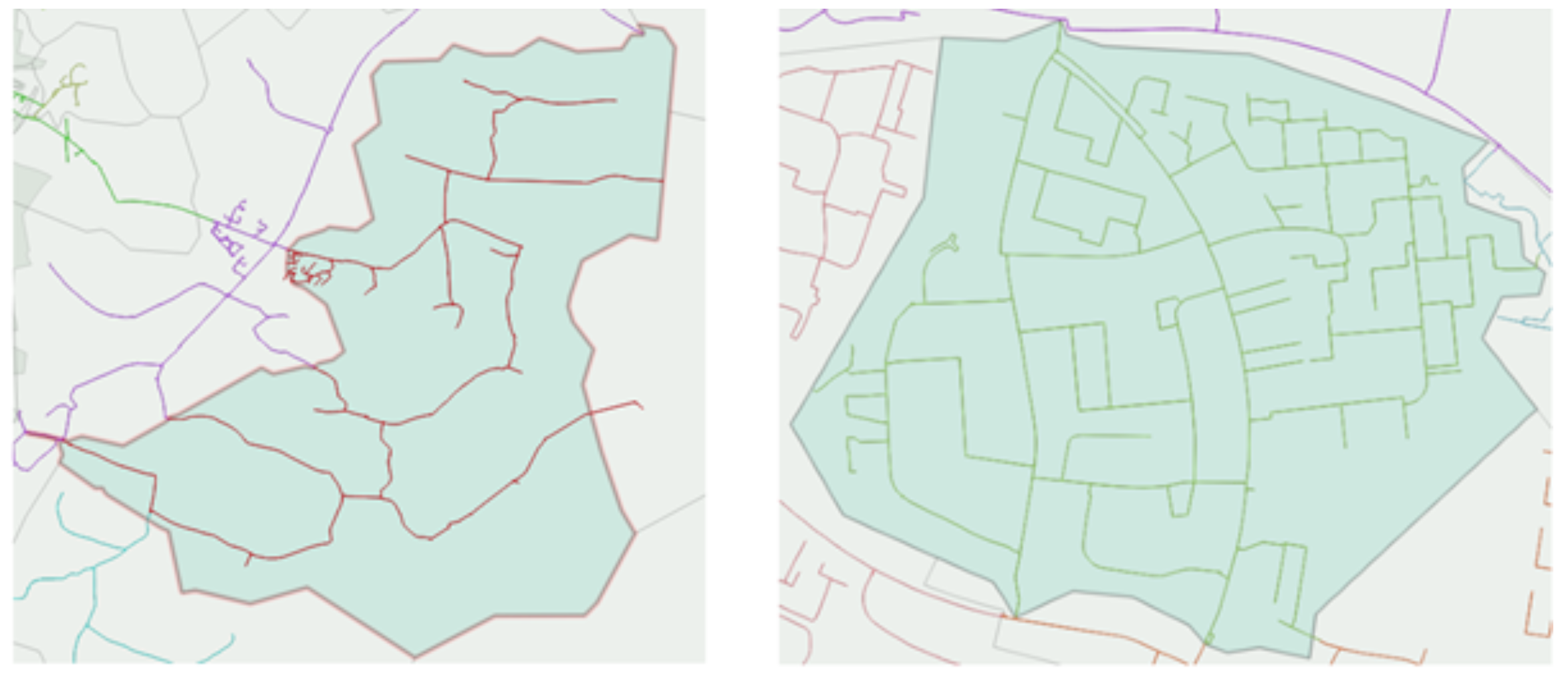
Consider the difference between the two DMA networks shown in Figure 4. It’s clear from visual inspection that each of these networks will exhibit different characteristic head loss behaviours. Due to the ‘branched’ nature of the network shown in Figure 4a, there is only one path along which water flows between any two points, whereas the ‘looped’ (or grid-like) nature of the network shown in Figure 4b introduces multiple parallel flow paths which will affect the head loss response to a given change in demand. If we could quantify this quality of ‘loopedness’ and find a way to phrase the problem to the computer, this would also help to quantify the resilience of the DMA to mains failures in terms of link criticality, without having to run any models.
Figure 4a: A ‘branched’ DMA network Figure 4b: A ‘looped’ DMA network
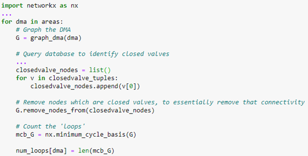
Again, there is a concept from graph theory which can help us here. A loop in a graph is referred to as a cycle, and the ‘minimum cycle basis’ of a graph is a set of subgraphs comprising all of its smallest loops which are not themselves bisected by an edge. In other words, by asking the computer to count the number of cycles in the minimum cycle basis, we can count the number of loops in a DMA.
Figure 5 demonstrates how simply this can be accomplished in Python using Networkx, with the function minimum_cycle_basis(G). For the DMAs shown in Figure 4, the analysis gives a score of 0 for the ‘branched’ network and 24 for the ‘looped’ network.
Figure 5: Python coding example for counting ‘loops’ in a network
Identifying flow paths and estimating head loss
Earlier there was a reference to the applications of graph theory in route planning for GPS navigation, which is accomplished using a path-finding algorithm, such as Dijkstra’s algorithm. Given that a key concept of our analysis is to monitor the head loss between two points on the network, it would be useful to know about the physical characteristics of the flow path. Based on the pipe characteristics, we can then estimate the expected head loss range to improve the detection of anomalies. Networkx includes an implementation of Dijkstra’s algorithm in the shortest_path_between function, which has allowed us to automate the tracing of flow paths and retrieval of data such as pipe diameter and materials along each path for this purpose.
Conclusion
While the functionality offered by Networkx has proved very useful, we also encountered some limitations. The analogy of a water network as a graph does not lend itself well to analysis concerned with the attributes of pipes. In graph theory, nodes are the objects of interest to be modelled and links represent the relationships between them. This means that the algorithms in Networkx are very much set up for answering questions about nodes and their relationships (i.e. connectivity). When writing a routine for infilling missing pipe attributes from neighbouring pipes we found that Networkx made this quite difficult and opted for a non-graph-based approach instead.
Nevertheless, we’ve found that the graph functionality offered in Python by Networkx offers almost out-of-the-box solutions for several modelling problems, which we have incorporated into our automated data cleansing procedures. It will be interesting to learn more about its capabilities moving forward.