Python multiprocessing in Dynamo

Dynamo uses flow and pressure data to provide localised ‘areas of interest’ following a burst occurring. We have recently developed a new version of the system which implements the analysis in such a way that we can detect and localise burst events live throughout the day, as soon as the relevant flow and pressure data becomes available. This allows Dynamo to always be looking for new events and ensure our clients get insight as soon as possible.

When implementing a live system, the speed of processing becomes essential to its success. If we can’t import, analyse and report results from the data faster than the data is coming in, then it won’t work as a live system!

One of the ways in which we’ve optimised the performance of Dynamo, is by adopting concurrency where possible. Concurrency in this context means doing more than one thing at the same time, with the goal of improving performance by maximising the utilisation of server resources (e.g. CPU usage).

This blog will use examples of how multiprocessing has been used to speed up the time series data import to provide insight into how this can be achieved in Python. Rather than giving a comprehensive tutorial (of which several are available elsewhere), the aim here is to share some of our experiences in utilising the Python multiprocessing library and give an example of how it can be used to optimise the performance of some tasks.

Background

Firstly, a brief introduction to concurrency, in which some concepts have been simplified to make them more palatable and fit them in to this short blog. It was mentioned in the introduction that the method aims to maximise the utilisation of resources. There are two approaches to this:

• Multithreading
• Multiprocessing

In this post, we will be talking exclusively about multiprocessing.

A computer’s CPU has one or more processor cores, each of which can be thought of as being able to work on one task at a time, which it calls processes. Modern computers normally have multi-core processors on which we should be able to work on multiple tasks in parallel.

Your computer appears to be running hundreds of processes to run the applications you have open but in reality, each of its cores is only running one process at a time. It multitasks by switching between applications at opportune moments. However, using Python’s multiprocessing library, we can achieve true parallelism. We can apply this when performing the same operation many times over similar inputs, allowing us to improve performance.

For example, consider that we have a list of 4 numbers which we want to square. A program to solve this will run so fast that we don’t need to optimise its execution time, but it serves as a good example. A conventional approach might be to:

1. write/appropriate a function which accepts a single number as an argument and returns the square of that number; and
2. write some procedural code which uses a for loop to iterate over the list, executing the function on each element and appending the results to a second list.

Figure 1 shows how Python would execute this code on a quad-core computer. The running time of our program will be about 4 times as long as it takes to calculate the square of one number, as the numbers are squared one-by-one. We cannot start calculating the square of the second element before we’ve calculated the first, and so on.

Figure 1: Example of serial execution of a simple Python function

We can approach this problem differently by using the multiprocessing library:

Initialise a pool of (4) worker processes using the Pool class.

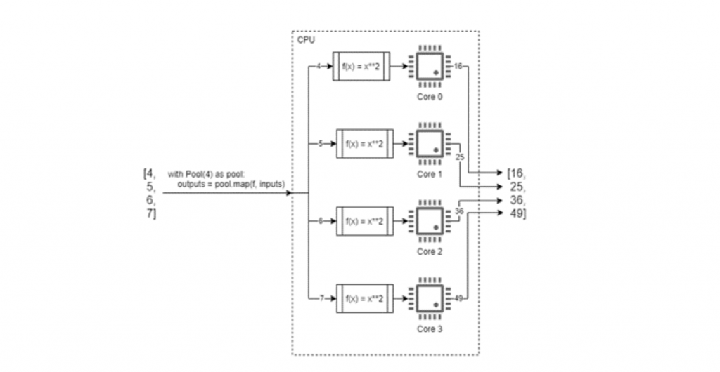
Use the map function to share the list of inputs to our function f across the 4 worker processes, each of which can be executed on separate cores (i.e. in parallel time), into a corresponding list of outputs.

Figure 2 shows how Python might execute this code on a quad-core computer. The running time of our program can potentially be much less than 4 times as long as it takes to square one number. It won’t quite execute 4 times as fast, due to system overhead associated with the parallelisation, but it will still be a lot faster.

Figure 2: Example of parallel multiprocessing of a simple Python function

What if we have more than 4 arguments? Well, we can still call map in the same way, and it will split up our list of inputs into chunks, which are shared out among the worker processes. Imagine each chunk forming/joining a queue in front of its worker process, from which the worker process will pick inputs one at a time until they have all been processed and mapped to their respective places in the outputs list.

The size of these chunks can be specified using the optional chunk_size parameter. Where this is not specified, the map function uses a heuristic approach to choose a suitable chunk size. This is based on the length of the argument list (how many inputs do we have to process?) and the number of worker processes in the pool.

But what is a suitable chunk size? It turns out that the answer to this question is really quite complex (refer to https://stackoverflow.com/questions/53751050/python-multiprocessing-understanding-logic-behind-chunksize), but for our purposes the answer is simply whatever runs the fastest!

Example optimisation

We will now look at an example of how we’ve optimised CPU utilisation in Dynamo.

Dynamo imports flow and pressure data which arrives thro an FTP server as .csv files. Each file normally contains flow and/or pressure data for a single timestamp which means that, on average, every 15 minutes we receive one file per logger. This can amount to a lot of files! Each time the time series data import runs, it must perform the same two operations on every file:

1. Read the file contents to extract the data (logger, channel, timestamp, value) and compose an SQL statement which can later be run to insert the data to the database.

2. Write the data to the database by executing the SQL statement composed in step 1.

To demonstrate how we can take advantage of concurrency in Python, let’s consider how to apply multiprocessing to the read_file function performing Step 1. In reality, this step in the end-to-end process is relatively fast compared to the subsequent data analysis and so its optimisation isn’t a big factor in Dynamo’s performance, but it’s a good example to see how we can apply multiprocessing.

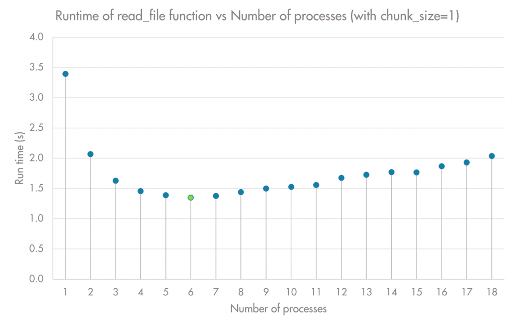
To facilitate this, we set up a test environment with 27,000 .csv files of time series data ready to be imported. Firstly, the chunk_size parameter was fixed at 1 and the number of worker processes in the pool swept from 1 to 6, which is the number of cores in our server’s processor. For each combination of parameters, the average run time from 5 sets of 5 tests, each set being conducted 5 seconds apart, was recorded. We were surprised to find that attempting to open a pool of 7 or more workers did not return an error as expected, so we continued the sweep up to 18 worker processes.

Figure 3: Run time of a read_file vs Number of processes (with chunk_size=1)

The results are presented in Figure 3. We can see that the run time is reduced considerably by the addition of the first few parallel workers, but that there are diminishing returns when reaching 5 and 6 workers. This is partly due to the increased parallelisation overhead incurred by more workers, and partly because by the time we reach 6 worker processors we’re executing on all cores, at least one of which is also switching between our worker process and other system/application processes. Beyond 6 workers, the run time begins to increase again. Again, this is because we can execute at most one process on each core, so our 7th process will be parked until a core is available (probably when one of our first 6 workers is finished).

So far, run time has been reduced by approximately 60%. To evaluate the effect of chunk size on performance and potentially find further optimisation, we wrote a script with an additional loop to perform the sweep described above across 8 different values for the chunk­_size parameter. This gives a total of 96 different combinations of parameters, each of which was run 25 times. The results are presented in a colour-scaled matrix in Figure 4 as run times in seconds, with the longest highlighted red and the shortest in green. The absolute minimum at 5 worker processes with a chunk size of 100 is also highlighted with bold white text.

Figure 4: Colour-scaled matrix of average run times in seconds of read_file function at 96 different combinations of parallelisation parameters

As mentioned earlier, the factors influencing optimum chunk size are complex, but we can draw some useful insights from the results. Perhaps most interestingly run time has been reduced by approximately 78%. The results show that increasing chunk size beyond a point (which depends on how many workers are in the pool) causes a reduction in performance. This is expected in extreme cases. For example, if we have 27,000 files to process and we specify a chunk size of 10,000 then the data will be split into three chunks of approximately 10,000, 10,000 and 7,000 in length. In this case, by forcing such large chunks we can only run on a maximum of 3 cores concurrently, which is reflected in the results where the run time increases in an approximately linear fashion for 4 or more worker processes. This is presumably due to the overhead required to spin up the surplus processes.

This prompts us to question why the optimum chunk size isn’t simply the number of arguments divided by the number of worker processes? In our case, for 5 processes this would be 5,400 but the optimum performance was recorded at a chunk size of 100.

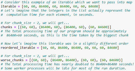
In a nutshell, this is probably because some arguments in our input list take longer to process than others. Whenever we use a chunk size of greater than 1, there is a risk that a chunk will contain at least one argument which takes significantly longer than the others in its chunk. This will essentially block processing of all subsequent arguments in the chunk until it has completed, which could lead to a situation where another worker process has finished its chunk and is now idle but is unable to help with the processing of the remaining arguments. In this situation we would not be fully utilising CPU capacity, and the run time will increase. An extreme example of this is given in Figure 5.

Figure 5: Example of how inappropriate chunking can lead to poor performance

By using a smaller chunk size, we combat this behaviour by reducing the average number of arguments for which processing will be held up by a large file in front of it in the queue (chunk). In other words, there is a performance benefit from the scheduling flexibility offered by small chunks. However, this benefit must be offset against the parallelisation overheads caused by Python and inter-process communication. The result of this is the optimisation that we see in Figure 4!

Conclusions and next steps

In a live event-driven system, quick processing is essential to avoid becoming overwhelmed by the volume of incoming data. Multiprocessing is one of the technologies we are leveraging to achieve rapid event response in Dynamo. In the example optimisation above, the average run time of the read_file function over the testing load was reduced by 78%. This demonstrates that by identifying tasks suitable for parallelisation and writing our programs slightly differently, we can maximise the utilisation of computing resources to improve performance.

It will be interesting to continue learning about how different methods of software implementation and architecture can help us to deliver live burst localisations and other valuable insights to our clients.