Dynamo, our flagship product, relies on frequent pressure data from logged points on the network to ensure it is truly dynamic. This means that the reliable communication of data from pressure loggers is fundamental to the work that we do.
Our clients’ logger data is typically sent every 30 minutes, giving a maximum of 48 call ins per day; any logger that does not call in for 3 consecutive days is labelled as ‘quiet’. It is important that the daily number of call ins are tracked for each individual logger, as it feeds maintenance activity and gives an overview of signal quality across the network. Signal quality can also be plotted in QGIS, adding a spatial element to the data, and allowing visibility of signal ‘blackspots’ and anomalies.
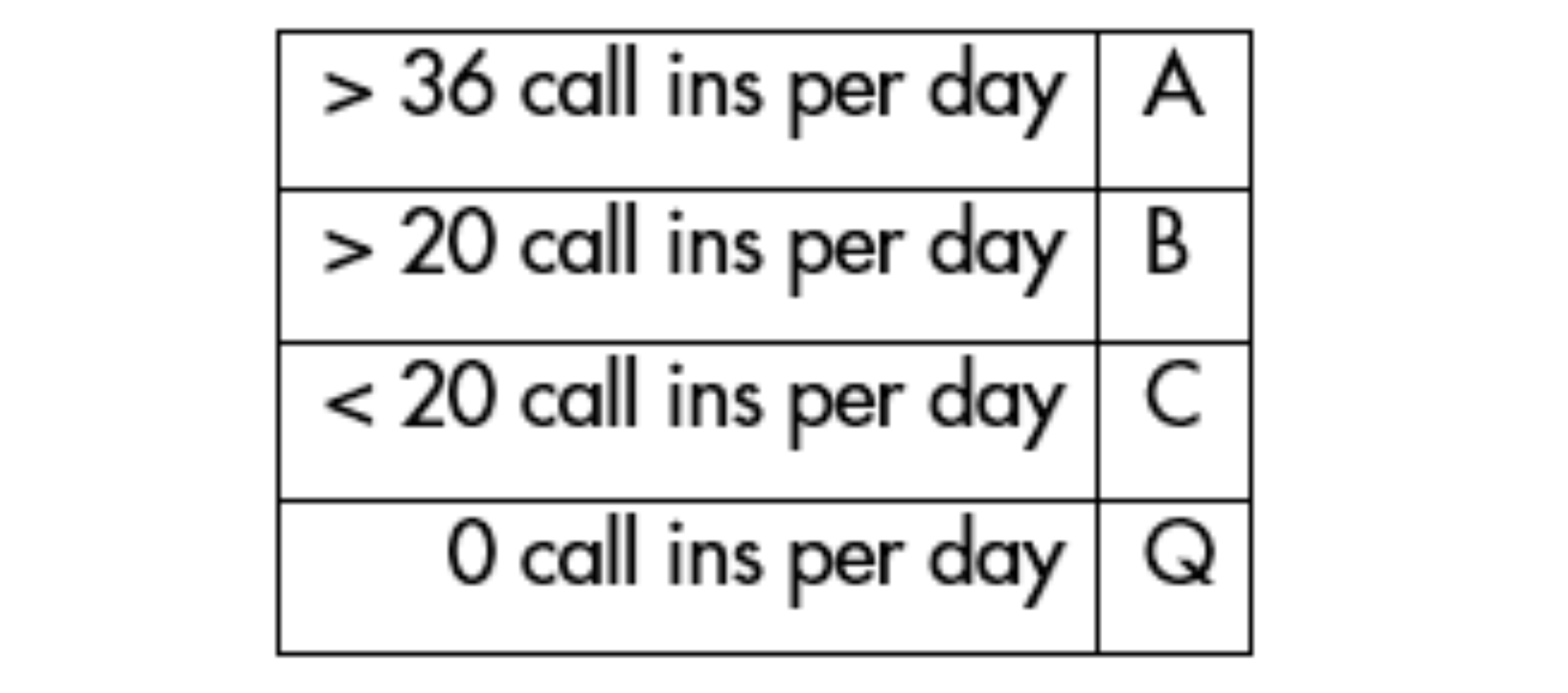
To help us understand areas of poor signal coverage we group the number of signal call ins per day into the following categories:
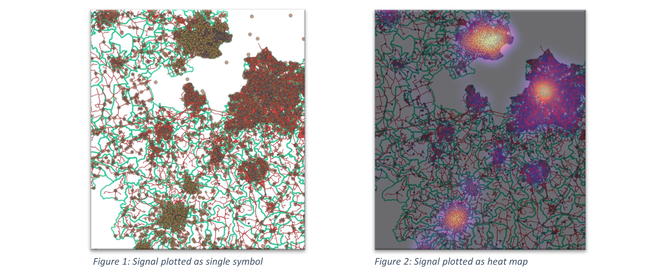
Figure 1 shows the data for June 2020 across the network when plotted in QGIS as single symbols. Using single symbols reduces the visibility of the network and makes it difficult to determine where the points of interest are due to the high density of data. In comparison, Figure 2 demonstrates how using a heat map to display the data allows for greater visibility of points of interest as well as ensuring that layers beneath (i.e. DMA polygons and logger site IDs) are still visible.
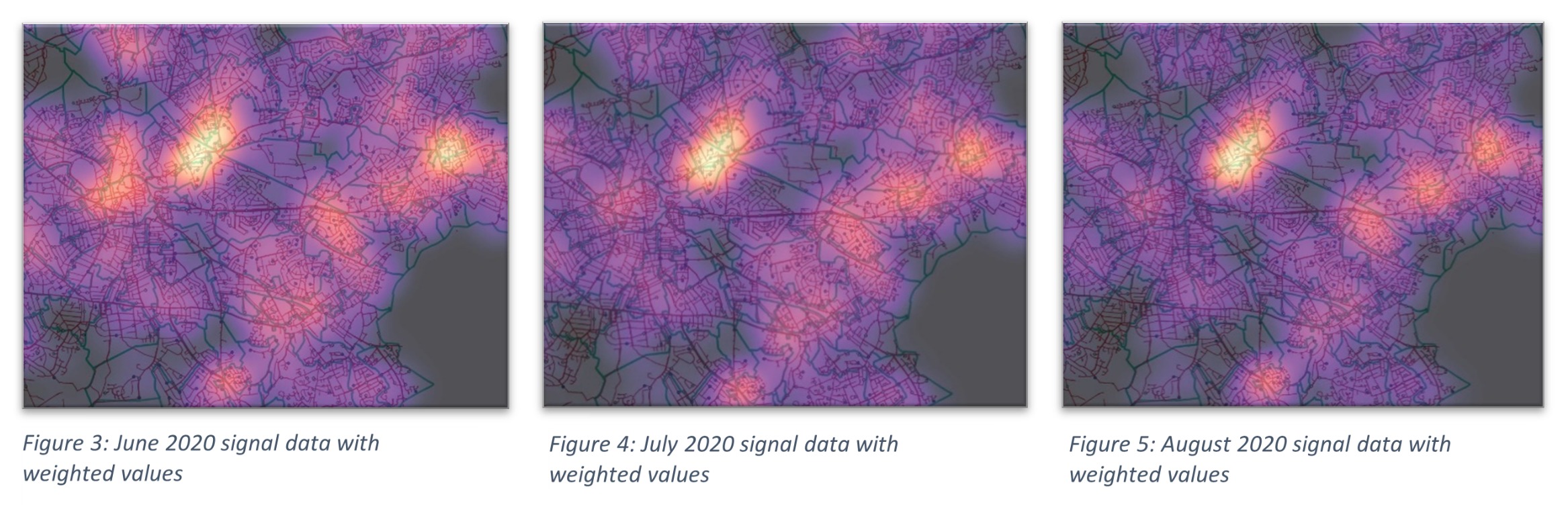
To differentiate points of interest even further, it is possible to add ‘weighting’ to each signal category within QGIS. For the plots below (Figures 3-5), the categories were weighted as follows:
These weights were chosen to bring attention to sites where the logger was quiet (Q) or was returning poor signal data (C).
As data is received daily, it is possible to track signal quality over time. Figures 3-5 show how poor signal areas can vary from month to month (30-day averages were taken for each month). Signal quality can be seen to improve over the time period in much of the chosen area. However, there is a clear ‘blackspot’ near the centre where loggers have had poor signal throughout. This area becomes more pronounced as the surrounding signal improves in August 2020, giving a clear point of interest for maintenance to take place.
By identifying these points of interest within a logger fleet, we can begin to search for trends across the network. These trends can be utilised to plan maintenance more efficiently; rather than having maintenance resource spread evenly across the network, designated resources can be strategically placed in areas that have historically had poor signal quality. Cutting down the travel time between jobs leads to a reduction in maintenance costs and an increase in productivity.
In areas that show persistent signal issues, QGIS plots can also be used to identify sites that could benefit from alternative solutions, such as integrating aerials into chamber lids, which would improve the signal quality in DMAs where logging is key to leakage detection. As heat mapping allows visibility of layers beneath, it is a simple task to identify hydrants that could be candidates for lid installation.
Continuing to track signal quality in the future will produce benefits by giving us a greater understanding of trends such as seasonality, mast signal strength fluctuations, and even how urban demographics can affect logger signal. By understanding how these issues affect the fleet we can ensure the best possible asset health for our clients whilst utilising quality pressure data to help reduce leakage.